9 Excel Formatting Techniques That Will Save You Time

Table of Contents

Quick Formatting
Wrap Text
Widen Columns
Format Painter
Format As Table
Conditional Formatting
Remove Duplicates
Custom Views
Symbols
Conclusions

Quick Formatting

I use-to spend a lot of time formatting the background colour of headings then making the text white. Changing the font and size and then trying to remember what my style was to apply to other Excel workbooks because I like to keep my formatting consistent with my business branding.

This process was taking me for ever and going back and forth finding Excel workbooks that had the formatting I liked or finding the notes where I had written the style attributes, was just becoming a nightmare until I noticed Cell Styles.

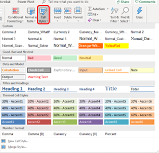
Yes, it was right in front of me for a long time. Cell Styles are found under the home tab.

1. Select relevant cells
2. Home tab
3. Select Cell styles
4. Choose the colour from the list
5. You can even create your own style

Keeping Zeros in front of product numbers can be tricky, as a facilitator with over 24 years’ experience with Microsoft Office products I have seen some work around for this one.

VLOOKUP FUNCTION ISSUES

Apostrophe in front of the number. This does keep the zeros in front but also treats it as text not a number. Which is fine it does let you perform calculations but if you are using it for other functions it may not work as those functions are looking for a matching format. For example, your VLOOKUP Function may not work out.

Type some text then the number, mmm sure but most of the time that’s not the look we are going for or it impacts on the outcome if you are then wanting to sort by numbers or need it for your Lookup Value when doing a VLOOKUP Function EG: INV 300, AMOUNT 300

If you are typing a mobile number, ABN, ACN or TAX File number and enter the spaces the zero in front will be retained.

CUSTOM NUMBER FORMATTING IN EXCEL

If the number, you need to type has NO Spaces then you will need the ultimate technique. Go to Custom Format or Press ” Ctrl 1″. Select Custom and enter a 0 for every digit you need displayed. If you need spaces or specific symbols include these.

Eg: 0000 enter 1 digit. 5 result will be 0005

000-00 enter 1 digit. 5 result will be 000-05

TEXT AND NUMBERS IN EXCEL

Let’s say you would like to display your number with SN in front of it but its such a chore to constantly type the text. Use Custom Format to display the “SN” text in front of your chosen numbers.

1. Go to Custom Format or Press Ctrl 1
2. Select Custom
3. Replace General with the following
4. Type “SN” 0000

Followed by a zero for every digit you need include any spaces or symbols such as – or /.

Type 5 result will be SN0005

This could be why when you try to use Text To Column to split the text from the number but it doesn’t display in the dialog box.

EMBEDDED COLOUR IN EXCEL CELLS

You may have come across a cell which has a colour applied to it and would like to remove or replace it with another colour. It also has the applied feature we discussed earlier of the text immediately followed by a specific number of digits. EG SN0005 and in blue.

The usual methods to remove or replace the formatting doesn’t work. Select the Cell, go to Home and change for Font Format to Black or another colour but it doesn’t work. What’s going one you may think.

CUSTOM FORMAT is going on.

Select the Cell/s and go to Custom Format (Ctrl 1) square brackets have been added to the front of the code to change it to the colour [Blue]

CUSTOM FORMAT COLOURS LIST IN EXCEL

Initially there are 8 Colours you can set in your Custom Format setting, they are:

[black] [white] [red][green] [blue] [yellow] [magenta] [cyan].

Wait there is more: 57 just make sure you spell colour the America way “color” no space between the number.

For Example, Color3 written in the Custom Format dialog box as: [color3]0000

Type the number 5 result 0005 in red.

CLEANING EXCEL FORMATS MADE EASY

We hear the words time poor thrown around and that includes when working with an Excel Spreadsheet. In the back of your mind as you’re working on your Excel Spreadsheet you think – there must be an easier and quicker way to get the job done. Formatting the spreadsheet and cleaning up the mess others have left behind is taking for ever. There is a quicker way. No, it’s not Delete, Delete that for emails – ha ha.

If you have a block of data that needs the formatting stripped back to Normal. Try Ctrl A this will select a block of data. From the Home tab select the Clear command then Select Clear Formats. This will leave behind the data but strip the Font, Size, Colour etc.

HOW CAN YOU DISABLE A HYPERLINK IN MICROSOFT EXCEL?

Importing data is quite a popular task to be used in conjunction with Microsoft Excel. If importing client or employee details, you might get and Email address, Website Address or links to social media. When you don’t need it to be active it can send you off accidentally to that email or web site causing delays and frustration.

Selecting the cells with the hyperlink can be tricky since every time you try and click on it to select it it’s going to shoot you off to the web site. Click one cell away from the hyperlinked cell and use keyboard shortcuts to select the data by holding the Shift key and your arrow keys. The Shift key selects but if you included the Ctrl key it will Select and jump blocks of data. In summary select one Cell away from the hyperlinked cell and Hold Ctrl Shift then tap the arrow keys.

Once you have the data selected go to the Home tab Select Clear and choose Clear Hyperlinks.

Still need help watch this video for instructions on how to retain zeros in front of numbers when using Microsoft Excel.

https://youtu.be/2LrpbpJPBFY

For more formatting concepts visit: 6 Useful Tips on Excel Formatting

Conclusion

To retain Zeros in front use spaces or symbols as your separator. For a mobile use spaces 0414 417 059 and the zero in front will remain. When it’s not possible to use symbols use the ‘ but keep in mind this technique will treat the number as text not a number. For best results go to Custom Formatting and enter a Zero for every digit you want to display.

To remove hyperlinks go to the Home tab select Clear then Clear Hyperlinks.

Still stuck, Book a face to face training session.
www.azsolutions.com.au
Sydney – Greater West Australia – Currans Hill

Wrap Text

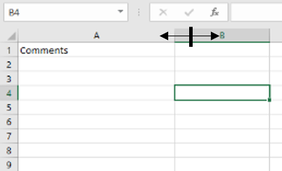
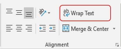
Wrap text is when you want to keep the column width at a specified size. It’s great for comments or notes. Start by setting the column to the width you would like by Dragging from between the column letters, your mouse pointer will change to a double headed arrow. Select the cell to do the wrapping on. Go to the Home Tab select Wrap Text.

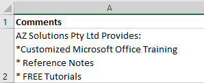
You might like to use a dash – or an Asterix * to represent a bullet point in your comments field, use wrap text and Alt Enter to keep the text in the same cell but in the next line down.

PC Users: Press Alt Enter.

Mac users: Press Option Command Enter.

Widen Columns

There are several techniques you can use to widen the columns in Microsoft Excel. Try double click between the column letters. Ensure you are getting a mouse pointer with a skinny little cross not the down arrow that will select the entire column.

When widening a column to a specific width, keep in mind the width is in characters and not in cm, mm or pixels. Position your mouse pointer between the column letters until you have the skinny little cross and then drag you will see the numbers display.

Are you the type of person who knows what they want and how they want to see it, try Right Mouse Click instead and select column width, type the no of characters wide you would like for example 20. The Column width will now be 20 characters wide.

Format Painter

We spend a lot of time making our Excel spreadsheets look good. At times someone else has done the hard work picking the correct colour, font, size etc and all you may be wanting to do is to re-apply exactly what they have done.

First select the text that already has the formatting you want, go to the Home Tab and select “Format Painter“. This is where most people say, yeh, yeh I know what to do.

Well I bet you pressed the Format Painter BUT only ONCE. Ok, try this click on the Format Painter TWICE, get trigger happy (DOUBLE CLICK) instead. The Format Painter will now stay on so you can apply to other text. When you would like to stop press the Format Painter again or press ESC.

Format As Table

Format as Table feature is not just pretty colours data is kept together as you enter it. This feature turns on the Freeze Pane, Filters, Colours for every second row and keeps your total together.

Found under the Home tab next to Conditional Formatting. It’s great with Pivot Tables if your data is continuously being added to. You could also use this feature in functions like the table component of a VLOOKUP Function.

The Default name for a table is “Table1” with no spaces in its name but you can change this to anything you like so long as there are not spaces in the name. Table1 is usable just like Range Names in functions.

New Records are created by pressing TAB on the last cell of the last record without disturbing your summary total. Records and column headings grow, keeping together as a database, making it a dynamic data set to use with Pivot Tables and charts. Saves the need for creating an Offset function. Ensure there are no blank columns or rows.

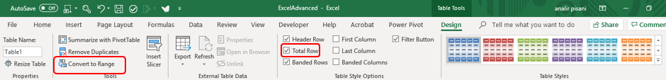
Tip: If you need to use Subtotalling you must turn off the Table Feature. Press Convert To Range.

1. Ensure your cursor is in the data set
2. Home Tab
3. Format As Table
4. Choose a Colour

Notice as you scroll down your column headers change from letters to what you had in the top row of your data set.

If this is not working for you then you have not selected a cell inside the data set and you will not be seeing the tab for Table Tools. Any formatting from before due to conditional formatting will not be affected.

If the colours are not showing according to what you selected, then select the cells and clear the formatting.

Clear formatting can be found in the Home tab on the far right.

Format Table For Mac

The Macintosh also has the feature of Format Table which has the benefits of:

• Freeze pane
• Sort/ Filter
• Totals Row
• Alternate row colours
• Data extending as you type in new Rows and Columns.

What’s different is naming your table. Whilst on a PC on the top left you have “Table1″ name, almost above the name box. The Mac does not.

For this on Mac you will need to Press the button for Rename (even though you haven’t named it yet.). Now give it a name.

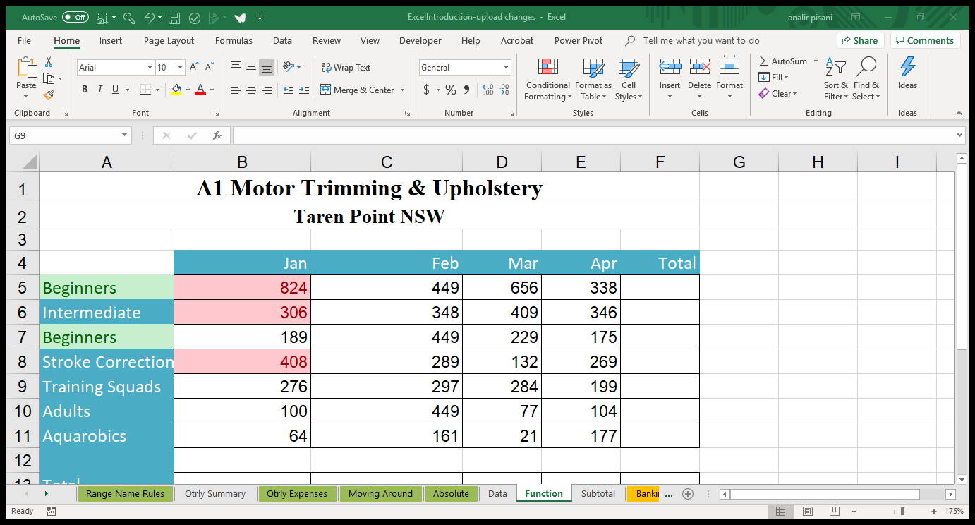
Conditional Formatting

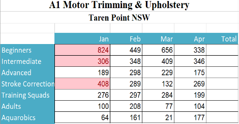
Conditional Formatting can be used to show you your standout sales reps or detect when stock is low. Help you pin point problem areas in the business using colour, symbols and graphs. It’s nice to know when you have reached your target with a splash of colour.

1. Select your cells to format with colour
2. Home Tab
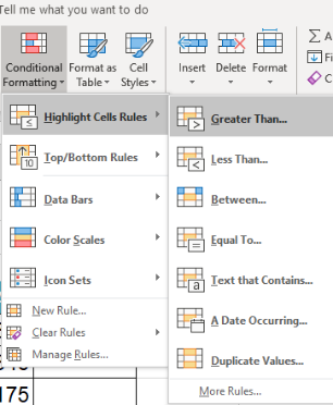
3. Conditional Formatting
4. Select highlight Cells Rules
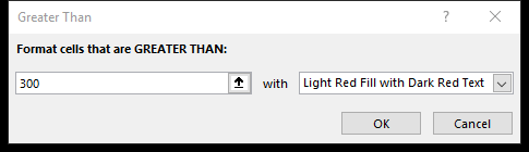
5. Greater Than
6. Enter eg 300 and Select the formatting

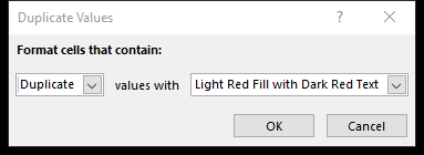
Highlighting Duplicate Values

Make duplicate values stand out. Check invoice numbers, Order numbers, Product codes don’t appear twice in your master list.

1. Select the cells to change in colour
2. Home tab
3. Conditional Formatting
4. Highlight Cells Rules
5. Duplicate Values
6. Choose your colour options
7. Note you can also select Unique values

Icons And Sets Conditional Formatting

It can be handing to display symbols to let you know if figures are higher or lower than a benchmark amount. When you use this feature, you will need to display a legend just like in graphs.

1. Select the Figures
2. Home Tab
3. Conditional Formatting
4. Icons and Sets
5. Choose your icons
6. Ensure you are still in at least one of the entries with an icon
7. Home Tab
8. Conditional Formatting
9. Manage Rules
10. Edit Rules
11. Press Alt Print Screen to take a snap shot of only the open dialog box
12. Then Crop

Remove Duplicated Data

Removing duplicates use to be hard work. You would have sorted data, created an IF function to test the row above to the one below and return Yes or No.

Well forget all that hard work all you need to do now is press a button make a few selections and you are done and dusted. Where is that magic button you ask – tune in next week for the answer, just kidding.

If you don’t quite need to remove duplicates but need to know if there are any and where in the lists they are, then use Conditional Formatting to highlight the duplicates.

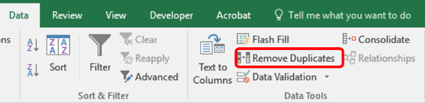
Sometimes we may have a list of, Account codes, Security pass code, Surnames or Departments where there should be no duplicates at all. Follow these steps to remove the duplicates.

1. Select the cells with the duplicate values
2. Go to Data tab
3. Select Remove Duplicates

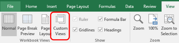
Custom Views

Custom view is a very useful tool when you find yourself changing the setting for printing your spread sheet, needing to change the page orientation, margins, page orientation, setting print area. Each sheet could have different needs. Follow the steps below

Option 1: Print all the data

1. Go to the View Tab
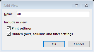
2. Select Custom View
3. Press the Add button
4. Type the Name all

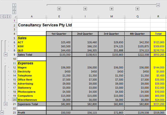
Option 2: Print only the Quarter

1. Set your spreadsheet up with Grouping
2. Select row 6 7 and 8 (the rows you want to hide)
3. Go to Data
4. Select Group
5. Repeat for column or rows to hide
6. Collapse and Expand your levels by pressing the + and – sign
7. Change any print settings – margins, page orientation
8. Now – Follow the steps in Option 1 and name it, Quarter

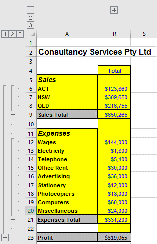
Option 3: Print only the Grand Totals

1. Collapse your levels
2. Change any print setting – margins, page orientation
3. Now – Follow the steps in Option 1 and name it, Grand Totals.

Fix Custom View Greyed Out

Items on the Ribbon become greyed out when you are in Edit mode in a cell. If you can see your cursor flashing in a cell, next to text or numbers you entered. The Ribbon will be greyed out. If you clicked in the formula bar, you are also in Edit mode.

If you look at the bottom left corner it will tell you what mode, you are in. Simply press Enter to exit this mode. If you press Ctrl Enter you will exit the mode but stay in the same cell ready to perform your formatting.

When you use added features like a graph, Pivot Table, Table or Slicers you will notice an extra tab in the Ribbon specific to this task and at times it may be disabled from using one feature while another is turned on.

There could be a few things going on sheets could be grouped or you could have the Format As Table feature turned on. If your sheets are grouped this will automatically disabling certain features in the Ribbon.

To Ungroup Sheets

Right Mouse Click on a sheet and Select Ungroup sheets. If that hasn’t solved your problem perhaps you have Tables active.

To Turn Off Format As Table

Ensure you are in the table data. You will see in the Ribbon a Table Tools tab, select Design and press Convert to Range. If Custom view is greyed out and there are no tables or sheets that are grouped.

Copy To New Workbook

Copy and paste the problem sheet to a new workbook. This usually clears out any underlying issues.

Mac users also have the feature of Format Table although some features are a little different visit my blog on Format Table for Mac.

Improved Symbols For Office 365

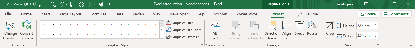
You can now insert your favourite icons like Disabled Icon, Toilet, Printer, Mobile, Finger Print Icon, Bed, Bin, Magnifier, Wi-Fi, Sound, Play, Battery Charging, Drop Pin, Lock, Hazards, Screen People, Party icons and much more into your Word, Excel, PowerPoint software packages.

They initially come in Black, but you can change them to whatever colours you like. Convert icons into SVG (Scalable Vector Graphics) – English ungroup them and change the colour of individual parts. Symbols command button remains, this looks to be an extension of Symbols.

1. Open Excel or Word
2. Go to Insert
3. Select Icons
4. Choose from the list and Insert
5. From the Graphics Tool tab
6. Select Format
7. Change colours or Convert to Shape to be able to change individual components.

Conclusions

Microsoft Excel has many interesting formatting tools apart from the basic Font, Size, Colour. I find the Format A Table Feature is often under utilised. Did you know that this feature is much more than a glorified pretty colours.

It turns on many features like Freeze Pane, Sort and Filter, Colours every second row, turns on a Total row for summing, adding or averaging. The best part is that it makes the data dynamic. In Conditional Formatting you can create formulas for your criteria to then apply colour.