Basic Excel Formulas and Functions You need To Know

Table of Contents

Basic Functions
Clean Up Functions
Naming Cells
Conclusions

Basic Functions

Functions follow a structured and there are over 300 functions pre-defined in Microsoft Excel eg = sum (A1:A12). When creating a function start with = then the function name followed by an open bracket, this bracket is important if you do not have it there is no function.

There are over 300 functions that Excel can do. The most popular ones are: Sum, Average, Max, Min and Count. The next most popular are IF and VLOOKUP.

Most importantly all functions begin with   =

They follow a structure = function name (range)

The sum function is =sum (A1:A12)

If the sum is going to be positioned under a range of figures ensure you select all the figures first, then press AutoSum. This will ensure you don’t miss out on any figures from the list.

Shortcut Key For AutoSum

Ensure that you have selected all the cells to be added before pressing your magic keystroke. The shortcut key for AutoSum in Excel is Alt =

AVERAGE

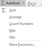
If you need to calculate the average of a range of figures. First select all the figures. Press the AutoSum command from the Home Tab but select the down arrow.

You should now see: SUM, AVERAGE, MAX, MIN, COUNT. This will put the result under the figures you selected. However if you would like to have the result positioned on a different sheet or in a cell not under the set of figures. Then Press = where you would like the result to be positioned followed by the FUNCTION NAME, AVERAGE remember the open bracket goes next in this order.

=FUNCTION NAME (

=AVERAGE(

Now select the range of cells it’s preferable you use your mouse to select the range of cells as oppose to typing them in and entering the colon symbol this is when you start to make too many mistakes. So select the cells with your mouse. You could press enter but I prefer if you get use to closing the bracket manually because when you start to create more complex FUNCTIONS, like a FUNCTIONS in side another FUNCTION you will be required to know how many closing brackets you need.

Your Average FUNCTION should look like this:

=AVERAGE(A1:A12)

When you are done always press Enter don’t get in the habit of clicking. When you are working in a FUNCTION and you click, it thinks you changed your mind about a cell reference and replaced what you had with what you just clicked on. So remember finish the FUNCTION with a closing Bracket and Press ENTER when you are done.

To do a MAX, MIN or COUNT FUNCTION replace the word AVERAGE with MAX

Note: If you Press = Ave you should get a list of functions that displays. You can press your up and down arrow keys on the keyboard to select the one you want, but when you are ready to select Press TAB not enter. Enter is used when you are finished.

Clean Up Functions

There are many functions in Excel over 300 in fact. There will be times when you will import data from other systems into Microsoft Excel and you will want to tidy up that data. For example, extra spaces at the beginning, end, or in between text is a popular scenario use the TRIM function to resolve this issue. This will ensure no errors when this data is used in other functions.

TRIM, UPPER, LOWER, PROPER, LEFT, RIGHT, MID, LEN, TEXT, CONCATENATE

TRIM

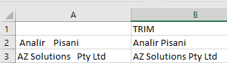
The trim function will take out extra space from the beginning, end or in between words.

=TRIM(CELL REFERENCE)

=TRIM(A1)

UPPER

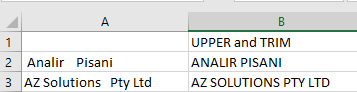
This function will change all the text in a cell to upper case. You may find that you will need to combine functions this is called created Nested Functions a function inside another function.

In this instance due to the spaces we will need to combine the TRIM Function with the UPPER Function.

=UPPER(CELL REF)

=UPPER(A1)

=UPPER(TRIM(a1))

For the functions LOWER and PROPER you can follow the same structure as above and simply replace the function name UPPER  with LOWER or PROPER.

The function PROPER capitalized the first letter of every word.

=LOWER(A1) or =PROPER(A1)

PROPER analir pisani will become Analir Pisani

excel courses sydney will become Excel Courses Sydney

LEFT

The function for LEFT will display the first x number of characters you nominate starting from the left. The functions starts with = followed by the Functions Name LEFT then the open bracket in that order.

=LEFT(

Select the cell which contains the text followed by a comma. The comma is important it says, now tell me how many characters starting from the left you would like to display followed by a closing bracket.

=LEFT(A1,3)

Analir =LEFT(A1,3) result is Ana

Remember if there is a space at the beginning of Analir then you will end up with na. This example below has an intentional space in front of Analir. Hence using the TRIM function is going to be necessary to tidy up the result to what you need.

Analir = LEFT(TRIM(A1),3)

RIGHT

The function for RIGHT is exactly the same as the function for LEFT with the exception that this function will return counting from the right.

MID

The function for MID will return characters from the middle you will need to select the cell with the characters to start from. You will then need to state the starting point by telling me how many jumps to the right. The count start from the number you stated eg 2 in my example jump 3 characters to the right from the letter n.  Followed by a comma then stating the no of characters you would like to display.

=MID(text,Start, No Characters)

Analir Pisani

=MID(A1,2,3) result is nal

LEN

The function for LEN means length of characters. This will count the number of characters in a cell including any spaces. This is great when you need to ensure that the product code is X no of characters long other wise it can’t be upload back into the system. Ensuring you have all the characters for your ABN, ACN, Bank Account no. SKU number, Batch numbers, ID’s and security passes.

All these fields often require to be a specific number of characters. We often interact with other systems like filling out forms on the web, import/export data to varies locations and if these fields don’t match a specific number of characters other related systems and functions might return errors.

Press = LEN then open bracket (

=LEN(A1)

analir result is 6

CONCATENATE

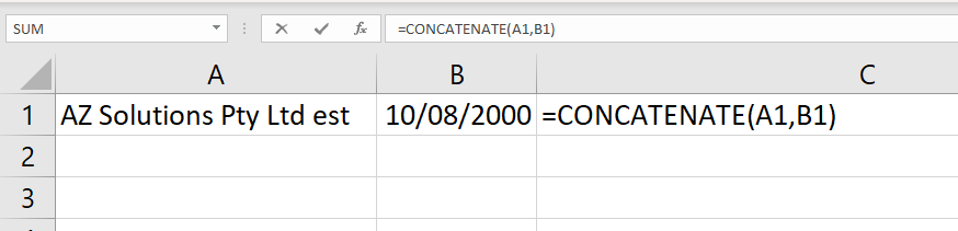
The CONCATENATE function joins together contents from other cells. For example you get 3 numbers and 4 text entries but they are in separate cells. You want to join them together to make up a new code. Perhaps you are wanting to perform a VLOOKUP function but there is no unique data, what you can do here is join a persons first and surname with an email address to make a unique field. If you join a text field with a data field or money field it will display in its raw format. For example the date 10/8/2000 will display as 36748. To retain the date formatting you will need to add the functions for TEXT, adding the TRIM function is also a good idea as this will clean up any extra spaces at the beginning of end of the cell.

AZ Solutions Pty Ltd est joined with 10-8-2019 will display as AZ Solutions Pty Ltd est36748

Join Cell A1 with B1

=CONCATENATE(A1,B1)

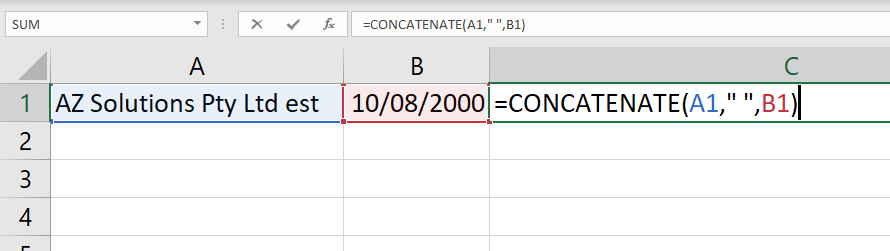
When joining cells there is no space between the contents of cell A1 and cell B1, using ” ” will give you a space between them. You can also enclose any symbol or text you want between the quote marks, for example “-” ,  “.” , “client name”.

=CONCATENATE(A1,” “,B1)

Joining cells can also be done by using the & sign. It is still a function so start with = followed by a cell ref then & and next cell reference.

Analir  in cell A1

Pisani in cell B1

=A1&B1 result is AnalirPisani

Notice there is no space between the two, add ” ” for a space between Analir and Pisani. Importantly you will need an other & sign. Think of the & sign as the glue between what is on the left and right of it.

=A1&” “&B1 result is Analir Pisani

Naming Cells In formulas And Functions

To make it easier to follow your functions you might like to create Range Name. Names that represent a range of cells then use that name in your function. Like the Table components of the VLOOKUP Function.

Using Range Names in Microsoft Excel will make it more efficient to navigate an Excel Workbook, but best of all use a Range Name in a function in place of the Cell References. What this does is make a lengthy function much more user friendly by making it easier to read. Take for example a VLOOKUP Function which is a popular function that matches data from one list to another then returns specified data from a column in the Master list.

Instead of reading: = VLOOKUP(A6,StockList!$A$1:$F$300,4,False)

In place of the table item you can use a Range Name like ProductList, notice there is no space in the Name, that’s important.

VLOOKUP(A6,ProductList,2,False) or = Sum(SalesTotals).

Another idea where you can use Range Names is in Data Validation Lists, or to make it easier to print reports you could create a Range Name that selects the area to be printed. There are several techniques you can use to create your range names use: Name box, Create From Selection, and Name Manager command button. You can use F5 to Go to the sheet it will select the cells that are in that range.

Rules When Naming Ranges

There are rules about Naming Ranges: – No Spaces is the big point to make as most people forget. The Range Name must start with a letter, no symbols, you can use text and numbers, but it can’t be the name of a cell for example: You Can’t use QTR1 as this is the name of a cell. The next big point that people forget is you must press ENTER otherwise you have not completed the steps and your Range Name will not work.

Create Range Names Using Name Box

1. Select the cell/cells
2. Type in the Name Box
3. Press Enter when finished
4. Ensure you have applied the rules for naming

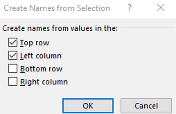
Create Range Names From Selection

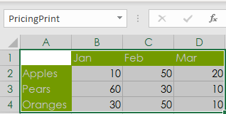
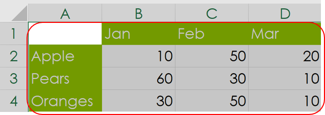
1. Select the group of cells including the heading labels on the Left Column and Top Row
2. Go to Formulas Tab
3. Press Create from Selection
4. You will be asked to confirm if the labels are on the Left Column or Top Row

Modify A Range Name

If data has been added to the list for this to be included in your Formulas and Functions, you will need to update the cell ranges.

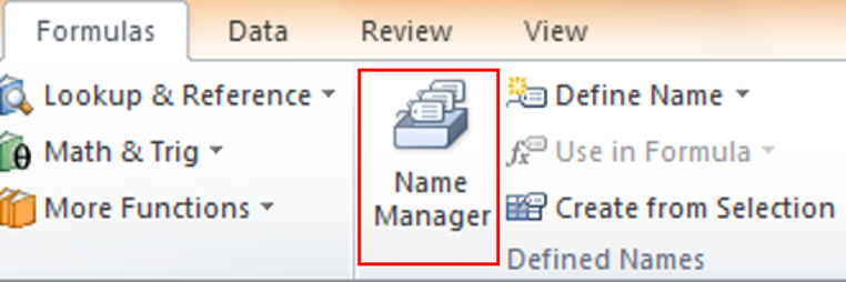
1. Formulas Tab
2. Defined Names Group
3. Name Manager
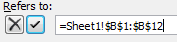
4. Make the change in the Refers to: Field
5. Press the Tick box to accept

Range Names In Functions

Perform a basic SUM Function by tying the Range Name where the range of cells would normally be positioned. Using Names in functions makes it easy to read back the formula or function. Especially for Nested functions like the IF Function.

1. Press =
2. SUM and Bracket (
3. =SUM(
4. You can type the Range Name if you remember it, or double click it
5. Press ) close bracket and enter

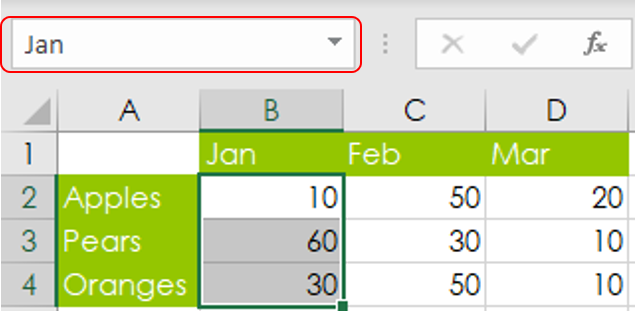
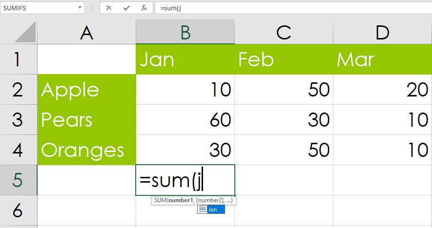
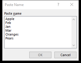
Perform a basic SUM Function by using F3 to insert the Range Name instead of typing it. This is helpful when you forget the first letter of the name you gave the Range Name.

1. Press =
2. SUM and Bracket (
3. =SUM(
4. Press F3
5. Select Jan from the list

Conclusions

Microsoft Excel has over 300 Functions the ones we use every day are SUM, AVERAGE, MAX, MIN, COUNT. Then there are what I call Clean up Functions like. LEFT, LEN, TRIM, UPPER, LOWER, PROPER, CONCATENATE AND TEXT.