Advanced Excel Functions
Table of Contents
Vlookup
Data Validation Lists
XLookup
IF Function
Nested IF Functions
Conclusions
Create A VLOOKUP Function
Great, you have been told you need to do a VLOOKUP. What is a VLOOKUP? When should I use it?
A VLOOKUP function in Microsoft Excel is a glorified copy and paste tool. It looks for a matching piece of information finds it in a table and brings back information it found from a specific column.
Imagine you have a massive set of data it goes on for ever, but you are only interested in a handful of columns from this data set. Use a VLOOKUP to make a smaller refined set of data and the data is still linked to the original so as updates occur you still have the latest information.
You could use a VLOOKUP for the purpose of making a smaller list and then using that list to create a PivotTable.
If you have an Invoice No, Order No, Product Id use the VLOOKUP function to bring back the description.
Lookup Functions
There are many types of lookup functions in Microsoft Excel, there is LOOKUP, VLOOKUP, HLOOKUP, CHOOSE, MATCH and INDEX. The VLOOKUP is the simplest and therefore the most popular. The V in VLOOKUP stands for Vertical lookup. The H in HLOOKUP stands for horizontal lookup.
Most times if your lookup value is presented horizontally you may have decided to select the data and perform a Copy/Paste Special Transpose then go ahead and do your VLOOKUP Function. If you only knew, you could have simply used the HLOOKUP function in Microsoft Excel.
When creating a VLOOKUP remember it will only return data from the right. If you need it to return data from the Left of the LookupValue use the INDEX function with the MATCH function together.
There are a few things to check before you can go crazy and start typing your VLOOKUP function. The table must be SORTED by the FIRST column in your Master List or table. Make sure you know the column number before you start typing your function.
The structure for the VLOOKUP is as follows.
=VLOOKUP(Lookupvalue,Table,Col Number,True or False)
You can replace the table data with a Range Name, this will help to understand what the VLOOKUP is doing.
False or 0 means: Exact match to Lookup value
True or 1 Means: Nearest Lowest match to Lookup value (True is the default)
If you need to find the nearest highest, then the VLOOKUP is not the right tool for you. Try a different function like INDEX and MATCH together.
VLOOKUP Function Errors
The Location of the LookupValue is important. It should be positioned in the first column of the start of your table. When cross matching data and extracting information from a specific column use VLOOKUP.
However, there are times when a VLOOKUP won’t do the job because it can only look to the right for the data to extract. If the lookup value in the Master List (Table) is located somewhere in the middle and you find yourself cutting and pasting the lookup value to the first column of the table.
That’s when you will need to use INDEX and MATCH function instead.
Take care of the lookup value and how it is formatted. If your lookup value is formatted for number and in the other area it is formatted as text or there is an extra space at the end. then the VLOOKUP will not work. To get rid of the extra space try the TRIM function.
What you can do to make your VLOOKUP function in Microsoft Excel so much easier to read is to use Range Names. Instead of selecting the Sheet and then the Master Data use a Range Name. You can also use Range Names in Data Validation Lists.
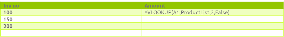
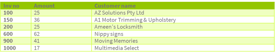
Scenario:
You have been asked to Match these invoice numbers to the master list and return the information in the amount columns.
Drop Down Lists
To avoid entering incorrect product codes, account names, surnames…
To limit options to a pre-populated list try creating a Data Validation List using Excel. In a separate sheet create a list of the data to display in the drop down, for example a list of department names or product descriptions.
You might like to then hide the sheet by right mouse clicking on the sheet name and selecting hide.
- Type a list of States
- Select the cell/s where you want the drop-down list to display
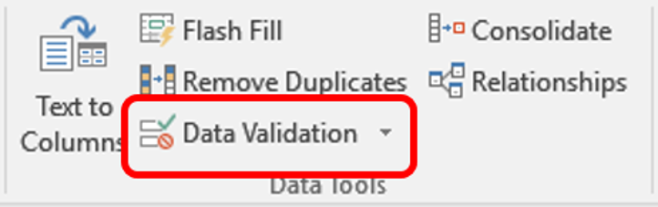
- Go to the Data Tab, Data tools group
- Select Data Validation
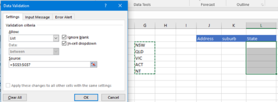
- In the Allow field
- Choose List form the drop-down arrow
- In the Source Field
- Select the range of cells with the States
- If you have given the States a Range name, then Press = and type the range name or Press F3 and select from the list
- You know have a drop-down arrow to select a state for your data entry.
YouTube Create A Data Validation List
Create A VLOOKUP Function
Great, you have been told you need to do a VLOOKUP. What is a VLOOKUP? When should I use it?
A VLOOKUP function in Microsoft Excel is a glorified copy and paste tool. It looks for a matching piece of information finds it in a table and brings back information it found from a specific column.
Imagine you have a massive set of data it goes on for ever, but you are only interested in a handful of columns from this data set. Use a VLOOKUP to make a smaller refined set of data and the data is still linked to the original so as updates occur you still have the latest information.
You could use a VLOOKUP for the purpose of making a smaller list and then using that list to create a PivotTable.
If you have an Invoice No, Order No, Product Id use the VLOOKUP function to bring back the description.
Lookup Functions
There are many types of lookup functions in Microsoft Excel, there is LOOKUP, VLOOKUP, HLOOKUP, CHOOSE, MATCH and INDEX. The VLOOKUP is the simplest and therefore the most popular. The V in VLOOKUP stands for Vertical lookup. The H in HLOOKUP stands for horizontal lookup.
Most times if your lookup value is presented horizontally you may have decided to select the data and perform a Copy/Paste Special Transpose then go ahead and do your VLOOKUP Function. If you only knew, you could have simply used the HLOOKUP function in Microsoft Excel.
When creating a VLOOKUP remember it will only return data from the right. If you need it to return data from the Left of the LookupValue use the INDEX function with the MATCH function together.
There are a few things to check before you can go crazy and start typing your VLOOKUP function. The table must be SORTED by the FIRST column in your Master List or table. Make sure you know the column number before you start typing your function.
The structure for the VLOOKUP is as follows.
=VLOOKUP(Lookupvalue,Table,Col Number,True or False)
You can replace the table data with a Range Name, this will help to understand what the VLOOKUP is doing.
False or 0 means: Exact match to Lookup value
True or 1 Means: Nearest Lowest match to Lookup value (True is the default)
If you need to find the nearest highest, then the VLOOKUP is not the right tool for you. Try a different function like INDEX and MATCH together.
VLOOKUP Function Errors
The Location of the LookupValue is important. It should be positioned in the first column of the start of your table. When cross matching data and extracting information from a specific column use VLOOKUP.
However, there are times when a VLOOKUP won’t do the job because it can only look to the right for the data to extract. If the lookup value in the Master List (Table) is located somewhere in the middle and you find yourself cutting and pasting the lookup value to the first column of the table.
That’s when you will need to use INDEX and MATCH function instead.
Take care of the lookup value and how it is formatted. If your lookup value is formatted for number and in the other area it is formatted as text or there is an extra space at the end. then the VLOOKUP will not work. To get rid of the extra space try the TRIM function.
What you can do to make your VLOOKUP function in Microsoft Excel so much easier to read is to use Range Names. Instead of selecting the Sheet and then the Master Data use a Range Name. You can also use Range Names in Data Validation Lists.
Scenario:
You have been asked to Match these invoice numbers to the master list and return the information in the amount columns.
Drop Down Lists
To avoid entering incorrect product codes, account names, surnames…
To limit options to a pre-populated list try creating a Data Validation List using Excel. In a separate sheet create a list of the data to display in the drop down, for example a list of department names or product descriptions.
You might like to then hide the sheet by right mouse clicking on the sheet name and selecting hide.
- Type a list of States
- Select the cell/s where you want the drop-down list to display
- Go to the Data Tab, Data tools group
- Select Data Validation
- In the Allow field
- Choose List form the drop-down arrow
- In the Source Field
- Select the range of cells with the States
- If you have given the States a Range name, then Press = and type the range name or Press F3 and select from the list
- You know have a drop-down arrow to select a state for your data entry.
YouTube Create A Data Validation List
IF Function
The IF function is a very important function because it is often used in combination with other Functions, such as, ISBLANK, ISTEXT, MATCH, AND, OR, NOT to name a few. More on Nested functions.
You will want to use an IF Function when you want one of two possible answers. For Example IF Cell A1 is equal to 10 then type the text “Sufficient Funds”, otherwise return a formula J20*.05.
Your response can be one of four types in the placeholder for TRUE and the placeholder for FALSE.
Structure for IF
=IF(Condition, True,False)
Explanation for Condition placeholder
Condition is where you get to ask your question but how?, what syntax do you use.
Use Comparison operators:
>
<
>=
<=
=
Functions for example: ISBLANK, ISTEXT, MATCH, AND, OR, NOT
Explanation for TRUE/FALSE placeholder
Example
=IF(A1=10,”Sufficient Funds”,J20-.05)
IF Function YouTube video
Nested IF Function
Nested IF Function YouTube video
Conclusions
Most popular function for cross checking data, looking up data from a master list, using it to create a smaller list for a Pivot Table is the VLOOKUP Function. Also try HLOOKUP or INDEX and MATCH Functions in Excel.
The XLOOKUP Function is the latest addition to Microsoft Excel, benefits include not limited by having the lookup value in the first column.
Can find a match which is nearest highest and find based on wildcard characters (*).
The XLOOKUP Function can find the last lookup value in a list instead of only the first. You now get a choice. Last or First occurrence to return.
Cell protection without having to set up cell protection.
It has an IFERROR component built in.
Microsoft Office Small Group Training Sessions
AZ Solutions delivers customized training courses in Sydney – Australia. We come to you. All you need is a board room, PC’s for each student and a TV/ Projector with a HDMI connection cable. Virtual Training sessional also available.
In our training sessions you are welcomed to bring examples of your work to class. We prefer it.
Call Now M 0414 417 059 visit www.azsolutions.com.au


